Finite Markov Decision Processes

WARNING!

Note - this is VERY EARLY DAYS! All of the files in the course with this warning are the raw, totally unprocessed notes that I generated during my first reading of “Reinforcement Learning: An Introduction”.

I’ll be converting these into proper course sections with wonderful embedded code that you can try out. I’m not there yet, but I wanted to develop all of this in the open.

Maybe you’ll find these notes interesting, but don’t expect anything special… yet!

Notes

There is not too much to go on here for programming exercises, which is nice. This is the shell for everything else. There’s really just the gridworld. The Python example does this by hardcoding everything in.

Can I make the gridworld really nice? Is there some interface that a game can satisfy…

I mean, embedding it in a webpage is the best thing I can do. You set up your gridworld and hit “train” and boom, it gives you something solid. Is this worth doing? Only if it’s easy!

Obviously good to go over the summary again on p. 69 before publishing anything here.

Historical Notes

This is covered on page 69, but maybe do some looking so we can give background on where these ideas came from.

Summary

• we get the model for what we’re going to talk about next, and a ton of the vocab. We’re NOT talking about how to set up problems to be solved by this framework… but now we know about rewards, discounting, action-value functions, state-value functions etc, and we have some hints about how we might implement this.
• The idea of how large the state space is obviously matters. For goofy examples like gridworld… it’s super easy to see what to do. For something more complicated, which is anything in the real world, anything really interesting, you’ve got to get more turbo and use the approximation methods in the second half of the book.
• But we get an intro to what training vs prediction are in this world. It is all about decisions that step the state of the world forward. And then you’ve got a hovering process, watching all of this and integrating information learned back into the relevant states. How far back do you get to remember? We’ll talk about that later.

Okay, this chapter introduces a bunch of different concepts, building up to this problem of… how do we model a system where different states present different opportunities?

• the finite markov decision process!

These state-dependent quantities are essential to accurately assigning credit for long-term consequences to individual action selections. (p. 47)

One q… they address this in chapter 17, but how do we go beyond the mathematical formalism? Are there things that you can only solve if you go beyond?

What is the “social psychology” field going to look like for AI and machine learning? How do things change when you can inspect inside the black box?

Next… the agent-environment interface.

This is a mathematical model, remember. You have some inner thing, the agent, that is interacting with a totally unknown world. I guess you could build a model of the world, but it’s assumed that the world is not inspectable except via the state representation you’ve built.

Something like this.

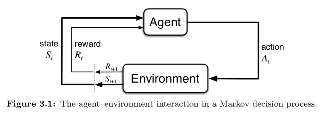
• then we introduce the function $p(s’, r | s, a)$, which defines the dynamics of the system. That term is interesting, since it shows up in all sorts of places. Dynamics means, the equation governing what the system will do next. In physics often the variable is time… here time is replaced by the idea of taking an action. That is what ticks the clock forward. This is really a function though.

The art is defining the boundary.

In practice, the agent-environment boundary is determined once one has selected particular states, actions and rewards, and thus has identified a specific decision making task of interest. (p. 50)

HUGE abstraction. Now lots of examples of stuff that fits into it.

Exceptions? when the state is incomplete and unknowable; random errors; or maybe… you wouldn’t want to use it when there is in fact a baked in physics model? Maybe not? That can come in later, as part of the thing calculating the value.

The reward hypothesis:

That all of what we mean by goals and purposes can be well thought of as the maximization of the expected value of the cumulative sum of a received scalar signal. (p. 53)

This is a little clunky. What it’s saying is that the goal is to maximize the total number of cocaine drips you’re going to receive in the future.

• “expected value of the cumulative sum” - you’re guessing. You also want the total number over time to be big, not just tomorrow.

So you have to craft an environment that produces rewards that send you toward a particular goal.

Of course this the alignment problem, right here. What if you fuck it up? This is called specification gaming: https://docs.google.com/spreadsheets/u/1/d/e/2PACX-1vRPiprOaC3HsCf5Tuum8bRfzYUiKLRqJmbOoC-32JorNdfyTiRRsR7Ea5eWtvsWzuxo8bjOxCG84dAg/pubhtml

That list is a bunch of amazing examples of the potential fuckups available.

The reward signal is your way of communicating to the robot what you want it to achieve, not how you want it achieved. (p. 54)

Then we talk about expected return, and how to discount items in the future. The whole trick is going to be how to pass back information about how the decision affected future states.

• episodic and continuing tasks are the same…

Then, the meat. All of reinforcement learning, most of it, anyway, is about estimating value functions.

State-value and action-value functions are the two big ones. You have some choices. What are you going to do next?

• Policy: a mapping from states to probabilities of selecting each possible action. The policy knows what it is possible to do next.

The policy uses the value function to decide what is best… but the value function has to assume some policy behavior to know what the policy is. Well, you don’t HAVE to… you can have an action-value function that does not assume. But state-value functions, if you just want to know “how good or bad is my current situation?” You need to know how you’re going to act.

If you perform a ton of trials, and visit each state a ton of times and keep track of what happened over many visits… Those are called “monto carlo methods”.

Bellman Equation

This comes up enough in reading that it needs its own section.

This is a recursive equation that gives the value of the current state as a sum of next states.

It states that the value of the start state must equal the (discounted) value of the expected next state, plus the reward expected along the way. (p. 59)

This is a different kind of dynamics.

The value function is the unique solution to its Bellman equation.

Then we get some examples… gridworld, golf.

Optimal

Can we get to a perfect one? You get this funky back and forth thing going between prediction and control. Often, a crappy policy can still generate the optimal value function, etc. 67-68 talk about this too.

I guess this section also talks about how it’s easy to compute an optimal policy once you have an optimal value function, and you can ping back and forth and see what’s going on.

Programming Exercises

• Demonstrate the interfaces required to implement this stuff, lock them all down and discuss the concepts using the interfaces as the hook.
• Gridworld?
• Golf example? maybe not…
• Note that when we code this puppy up, if we can come up with some way of indexing the state that is not just a unique ID, or where it came from, then we can start to piggyback with the afterstate example. If we can get to multiple tic-tac-toe pairs from the same spot…